dynamic programming approaches

When working with algorithms we will sometimes see that we can store values rather than recalculating, so that we don't have to solve for them past the first time.

Dynamic programming helps to reduce the number of recalculations in this fibonacci sequence.

Example Fibonnaci sequence

When n=0 or n=1, F(n) will return 1; and for other values of n the function F(n) will return F(n-1) + F(n-2).

Here F(n) represents our function itself unlike T(n) in recurrence relation in the previous exploration, where T(n) represents the time taken to solve problem of size n.

Algorithm

Fib(n):
    if n = 0:
        return 1

    else if n = 1:
        return 1

    else:
        return Fib(n-1) + Fib(n-2)

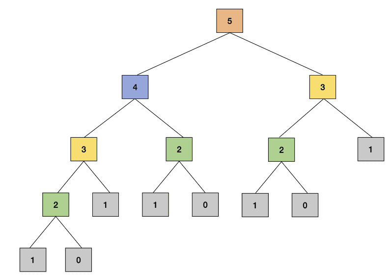
Call tree

This is a recursive call tree for n = 5 showcasing we have calculated the same result several times.

Speed and subproblems

We're repeating our work for the same subproblem, when we ask if we can speed this up we clearly can.

To avoid redoing the work of overlapping subproblems by storing the result after solving, we'll be able to run faster.

Two approaches to Dynamic Programming

This is a powerful algorithm design technique that can be used to solve problems that have strictly overlapping subproblems. There are two approaches that can be used:

• Top-down
• Bottom-up

Top-down approach

In this example the new variable FibMemo is a dictionary (key-value) that is used to look up the stored results of the subproblems we've seen.

This is also "seeded" with base case values.

If this is run for n = 2 we would get FibMemo = {0:1, 1:1, 2:2,}.

FibMemo = {
    0: 1,
    1: 1,
}


def Fib_top_down(n):

    if n in FibMemo:
        return FibMemo[n]

    FibMemo[n] = Fib_top_down(n-1) + Fib_top_down(n-2)

    return FibMemo[n]


print(Fib_top_down(5))

Time complexity

For every k, that belongs to [1, n] we calculate Fib_top_down(k) once.

T(n) = T(n-1) + theta(1)

This yields a complexity of Theta(n)

Secondary time complexity analysis

If we spend time to calculate only non-memoized values of n, n-1, ..., 1. Memoiozed calls are a constant time Theta(1) since we only have to look up the value in the structure.

Time Complexity = number of Subproblems * time/subproblem
                = n * theta(1)      [constant time, independent of "n"]
                ∈ Theta(n)

Slight tweak - no global scope

By passing reference to each subproblem we can avoid global scope.

def fib_top_down2(n, fibmemo=None):
    if fibmemo is None:
        fibmemo = {0:1, 1:1}
    if n not in fibmemo:
        fibmemo[n] = fib_top_down2(n-1, fibmemo) + fib_top_down2(n-2, fibmemo)

    return fibmemo[n]

Bottom-up approach

We solve smaller sub-problems first then combine the results until we solve the bigger problem.

This approach is also called 'tabulation' as we are constructing the table of results of all sub-problems until we reach the value of n for our problem.

For this we'll start with n=0, 1 then find n=2, 3 up to n

def fib_bottom_up(n):
    fib_table = [0]*(n+1)

    fib_table[0] = 1
    fib_table[1] = 1

    for i in range(2,n+1):
        fib_table[i] = fib_table[i-1] + fib_table[i-2]

    return fib_table[n]

Time complexity analysis

We're executing a for loop for range n, this will be Theta(n)

Comparing top-down and bottom-up approaches

• Top-down -
  • Start with the bigger problem and go down to the base case
  • We store the solution of the subproblems in extra memory space to avoid recomputing
  solutions
  • This is implemented typically with recursion
• Bottom-up -
  • We start with the base case and solve bigger problems as we progress to
  the actual problem (n)
  • This is typically an iterative approach that builds up the solution
  of the sub-problems and stores the solution in extra memory space