analysis of algorithms

Analyzing algorithms comes in a set of steps, followed by some mathematical concepts for presenting pseudocode as mathematical formulas to objectify.

Pseudocode

An important step of the algorithms discussion is determination of pseudocode to use as a "middleground" between a higher level programming language and the Big-O math.

Example

This is a linear search algorithm written in pseudocode.

Linearly search for an element k in an array A[0...n-1]

Note: Sometimes for assignment <- or := is used.

LinearSearch(A[0...n-1],k)
    i = 0
    while i < n and A[i] != k
        i = i+1
    if i<n return "Key found"
    else return "Key not found"

Time complexity

Determining the best algorithm for a problem requires determining answers to the time complexity and the space complexity of the function.

Running time

Identifying efficiency (running time) is important. Running time is a parameter of n where n is the input size of the algorithm, for BubbleSort n is the input array.

The running time is expressed as a function of T(n).

The choice of appropriate parameters that would impact efficiency depends on the function and the problem.

Order of growth

Writing the function of T(n) for run time looks at how many times each algorithm operation is executed.

                                            time to execute           execution
                                            instruction                 count
def PrintHelloNTimes(n):                        t1                        1
    print("Start printing Hello in a Loop")     t2                        1
    for i in range(n):                          t3                      n + 1
        print("Hello")                          t4                        n
    print("End printing Hello")                 t5                        1

Time to execute T(n) is:

T(n) = t1*1 + t2*1 + t3*(n+1) + t4*(n) + t5*1
T(n) = (t3+t4)*n + (t1+t2+t3+t5)

This running time is subbed as T(n) = an+b where a and b are constants that depend on the execution time of each line. where a = (t3+t4) and b = (t1+t2+t3+t5).

Since T(n) is a form of an + b we can say T(n) of PrintHelloNTimes as a linear function of n.

Example with Bubble-sort:

Bubble-sort(a)
 1 for i = a.length() downto 0                ------------------(n+1) * t1
 2     for j = 0 to i-1                       ------------------(n   +   n-1  +  n-2  +.....+1)*t2
 3                if a[j]>a[j+1]              ------------------(n-1  +  n-2  +  n-3  +.....+1)*t3
 4                         swap(a[j],a[j+1]); ------------------at most (n-1  +  n-2   +  n-3  +.....+1)*t4
                 end if

For lines 3 & 4:

When i = 0:
- j = 0 to -1. # j loop will not enter in this case.
when i =1:
- j = 0 to 0 # even in this case loop will not be entered.
when i =2:
- j = 0 to 1 # loop will be executed for j = 0
when i = n
- j = 0 to n-1 # loop will be executed for j=0,1,2,...,n-2

This is known as a quadratic function or n^2. When T(n) = an^2 + bn + c for simplifying analysis we can consider only the an^2, since the other terms are not as large of an n.

T(n) ~ n^2

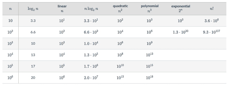
Example growth with the size of the Bubble-sort algorithm:

Runtimes of different Big-O times

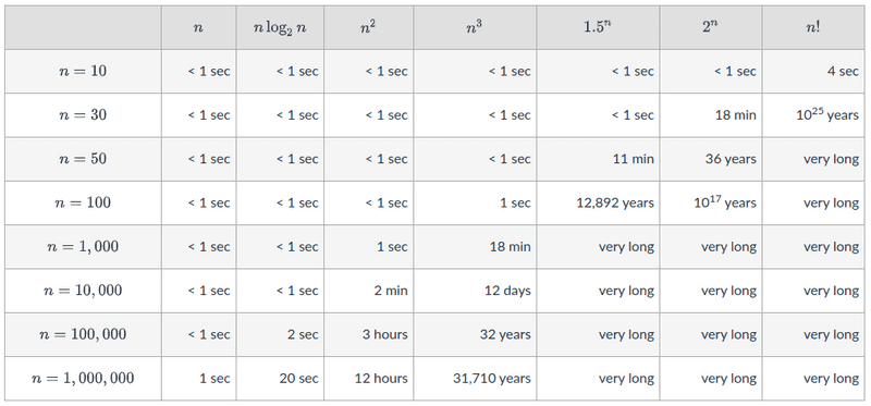
Below is a good table that illustrates the runtimes of different n sizes at different Big-O complexities (ex: n, n^2)

Example runtime complexity changes at different O's:

This of course is graphable like so: